Graph traversal features have been introduced in Solr 6 releases. These powerful features enables Solr users to run expressions that traverses graph structures in order to introduce or extract useful information. These graph traversal features are particularly useful when data is already indexed into Solr and light graph operations are required especially on top of text search. Before proceeding, a basic knowledge of Solr and graph structures is required.
Solr traversal implementation uses Breadth First Search (BFS) to perform graph traversal which is more suitable for solving search problems than its counterpart Depth First Search (DFS). It is also possible to combine graph traversal with other search or streaming operations.
In this post, we are going to explore basic graph visualization introduced in Banana v1.7. To visualize a graph in Banana, there must be at least a collection indexed into Solr with two fields: from and to that represent the adjacency matrix or, in other words, the edges of the graph. Alternatively, two collections can be used to visualize the graph: a main collection which is configured in the dashboard settings and an additional graph collection that stores the graph matrix. The main collection will be joined with the graph collection to retrieve node labels.
The Dataset
E-commerce sites usually display related products that other users bought along with the currently displayed one and Amazon is leading in this domain. Amazon product dataset published by the University of California, San Diego1 (UCSD) contains these data: the products and their related also-boughts. The dataset contains 9,430,088 products, each product in the dataset is represented by one non-strict JSON line. In order to index the dataset, a simple transformative pre-processing has to be performed. The preprocessing consists of two steps:
- Convert the non-strict JSON to strict JSON so that it can be correctly parsed
- Extracting a subset of the features from the JSON dataset and transforming it to CSV for indexing
- Building a graph matrix from
related.also_boughtfield
Preprocessing
The first step can be done using the script published on the author’s page. For the second and third steps, the following Python scripts can be used:
import json
import csv
import sys

# JSON to CSV

row = []
counter = 0

with open('metadata.strict.json') as metadata:
  with open("products.csv", mode='w') as products_csv:
    csv_writer = csv.writer(products_csv)
    csv_writer.writerow(['asin_s', 'title_s', 'title_t', 'description_t', 'price_f', 'imUrl', 'brand_s', 'categories_ss'])

    for l in metadata:
      product = json.loads(l)
      row = []
      row.append(product['asin'])
      if 'title' in product:
        row.append(product['title'])
        row.append(product['title'])
      else:
        row.append('')
        row.append('')

      if 'description' in product:
        row.append(product['description'])
      else:
        row.append('')

      if 'price' in product:
        row.append(product['price'])
      else:
        row.append('')

      if 'imUrl' in product:
        row.append(product['imUrl'])
      else:
        row.append('')

      if 'brand' in product:
        row.append(product['brand'])
      else:
        row.append('')

      if 'categories' in product:
        categories = []
        for category in product['categories']:
          categories.append(category[0])
        row.append(','.join(categories))
      else:
        row.append('')

      counter += 1
      if counter % 100 == 0:
        sys.stdout.write("Progress: %d   \r" % (counter) )
        sys.stdout.flush()

      csv_writer.writerow(row)
# Build adjacency matrix
import json
import csv
import sys
row = []
c = 0
with open('metadata.strict.json') as metadata:
with open("also_bought.csv", mode='w') as co_purchase_csv:
csv_writer = csv.writer(co_purchase_csv)
csv_writer.writerow(['from_s', 'to_s'])
for l in metadata:
c = c + 1
try:
product = json.loads(l)
if "related" in product:
if "also_bought" in product['related']:
row = []
for asin in product['related']['also_bought']:
csv_writer.writerow([product['asin'], asin])
if c % 100 == 0:
sys.stdout.write("Progress: %d \r" % (c) )
sys.stdout.flush()
except:
print(l)
Now we have the data ready to be indexed. Create two collections: products and also-bought, and index the data using post command shipped with Solr. Also, install Banana v1.7 if it’s not installed. Refer to the previous post for more details.
Creating the Dashboard
To create the graph panel and visualize products and their corresponding also-boughts, navigate to http://<solr-host:solr-port>/solr/banana/src/index.html and configure the dashboard collection to be products collection. Remove the default time-picker panel and time filter then create a new graph panel using the following settings:
- Title: Also-bought
- Label field:
title_s - Join_field:
asin_s - Root nodes: 5
- Graph collection:
also-bought - From field:
from_s - To field:
to_s
Close the dialog and the panel should render something similar to this:
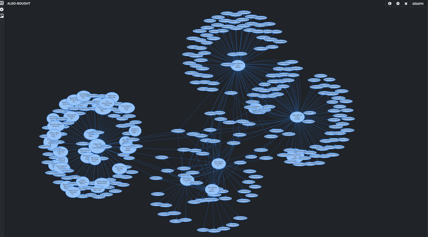
Immediately, it is noticed that products are formed in clusters. Few products have a significant number of also-bought products which means that customers who bought these central products tend to buy other products with them2. Experimenting with search terms, using the search panel, depicts similar graphs for the specific search terms. You may also add Sort and specify Sort Order parameters to further refine the graph.
Note: Root nodes parameter is the number of root nodes, based on the search terms used to traverse the graph.
1. R. He, J. McAuley. Modeling the visual evolution of fashion trends with one-class collaborative filtering. WWW, 2016
J. McAuley, C. Targett, J. Shi, A. van den Hengel. Image-based recommendations on styles and substitutes. SIGIR, 2015
2. Graph panel in Banana 1.7 traversal depth two levels